Integral
From Wikipedia, the free encyclopedia
This article is about the concept of definite integrals in
calculus. For the indefinite integral, see
antiderivative. For the set of numbers, see
integer.
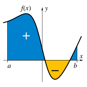
A definite integral of a function can be represented as the signed area of the region bounded by its graph.
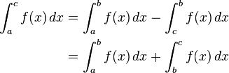
Integration is an important concept in mathematics and, together with its inverse, differentiation, is one of the two main operations in calculus. Given a function f of a real variable x and an interval [a, b] of the real line, the definite integral
-

is defined informally to be the signed area of the region in the xy-plane bounded by the graph of f, the x-axis, and the vertical lines x = a and x = b, such that area above the x-axis adds to the total, and that below the x-axis subtracts from the total.
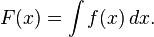
The term integral may also refer to the related notion of the antiderivative, a function F whose derivative is the given function f. In this case, it is called an indefinite integral and is written:
-
However, the integrals discussed in this article are termed definite integrals.
The principles of integration were formulated independently by Isaac Newton and Gottfried Leibniz in the late 17th century. Through the fundamental theorem of calculus, which they independently developed, integration is connected with differentiation: if f is a continuous real-valued function defined on a closed interval [a, b], then, once an antiderivative F of f is known, the definite integral of f over that interval is given by
-
Integrals and derivatives became the basic tools of calculus, with numerous applications in science and engineering. The founders of the calculus thought of the integral as an infinite sum of rectangles of infinitesimal width. A rigorous mathematical definition of the integral was given by Bernhard Riemann. It is based on a limiting procedure which approximates the area of a curvilinear region by breaking the region into thin vertical slabs. Beginning in the nineteenth century, more sophisticated notions of integrals began to appear, where the type of the function as well as the domain over which the integration is performed has been generalised. A line integral is defined for functions of two or three variables, and the interval of integration [a, b] is replaced by a certain curve connecting two points on the plane or in the space. In a surface integral, the curve is replaced by a piece of a surface in the three-dimensional space. Integrals of differential forms play a fundamental role in modern differential geometry. These generalizations of integrals first arose from the needs of physics, and they play an important role in the formulation of many physical laws, notably those of electrodynamics. There are many modern concepts of integration, among these, the most common is based on the abstract mathematical theory known as Lebesgue integration, developed by Henri Lebesgue.
History
Pre-calculus integration
The first documented systematic technique capable of determining integrals is the method of exhaustion of the ancient Greek astronomer Eudoxus (ca. 370 BC), which sought to find areas and volumes by breaking them up into an infinite number of shapes for which the area or volume was known. This method was further developed and employed by Archimedes in the 3rd century BC and used to calculate areas for parabolas and an approximation to the area of a circle. Similar methods were independently developed in China around the 3rd century AD by Liu Hui, who used it to find the area of the circle. This method was later used in the 5th century by Chinese father-and-son mathematicians Zu Chongzhi and Zu Geng to find the volume of a sphere (Shea 2007; Katz 2004, pp. 125–126).
The next significant advances in integral calculus did not begin to appear until the 16th century. At this time the work of Cavalieri with his method of indivisibles, and work by Fermat, began to lay the foundations of modern calculus, with Cavalieri computing the integrals of xn up to degree n = 9 in Cavalieri's quadrature formula. Further steps were made in the early 17th century by Barrow and Torricelli, who provided the first hints of a connection between integration and differentiation. Barrow provided the first proof of the fundamental theorem of calculus. Wallis generalized Cavalieri's method, computing integrals of x to a general power, including negative powers and fractional powers.
Newton and Leibniz
The major advance in integration came in the 17th century with the independent discovery of the fundamental theorem of calculus by Newton and Leibniz. The theorem demonstrates a connection between integration and differentiation. This connection, combined with the comparative ease of differentiation, can be exploited to calculate integrals. In particular, the fundamental theorem of calculus allows one to solve a much broader class of problems. Equal in importance is the comprehensive mathematical framework that both Newton and Leibniz developed. Given the name infinitesimal calculus, it allowed for precise analysis of functions within continuous domains. This framework eventually became modern calculus, whose notation for integrals is drawn directly from the work of Leibniz.
Formalizing integrals
While Newton and Leibniz provided a systematic approach to integration, their work lacked a degree of rigour. Bishop Berkeley memorably attacked the vanishing increments used by Newton, calling them "ghosts of departed quantities". Calculus acquired a firmer footing with the development of limits. Integration was first rigorously formalized, using limits, by Riemann. Although all bounded piecewise continuous functions are Riemann integrable on a bounded interval, subsequently more general functions were considered—particularly in the context of Fourier analysis—to which Riemann's definition does not apply, and Lebesgue formulated a different definition of integral, founded in measure theory (a subfield of real analysis). Other definitions of integral, extending Riemann's and Lebesgue's approaches, were proposed. These approaches based on the real number system are the ones most common today, but alternative approaches exist, such as a definition of integral as the standard part of an infinite Riemann sum, based on the hyperreal number system.
Historical notation
Isaac Newton used a small vertical bar above a variable to indicate integration, or placed the variable inside a box. The vertical bar was easily confused with  or
or  , which Newton used to indicate differentiation, and the box notation was difficult for printers to reproduce, so these notations were not widely adopted.
The modern notation for the indefinite integral was introduced by Gottfried Leibniz in 1675 (Burton 1988, p. 359; Leibniz 1899, p. 154). He adapted the integral symbol, ∫, from the letter ſ (long s), standing for summa (written as ſumma; Latin for "sum" or "total"). The modern notation for the definite integral, with limits above and below the integral sign, was first used by Joseph Fourier in Mémoires of the French Academy around 1819–20, reprinted in his book of 1822 (Cajori 1929, pp. 249–250; Fourier 1822, §231).
Terminology and notation
The simplest case, the integral over x of a real-valued function f(x), is written as
-

The integral sign ∫ represents integration. The dx indicates that we are integrating over x; x is called the variable of integration. Inside the ∫...dx is the expression to be integrated, called the integrand. In correct mathematical typography, the dx is separated from the integrand by a space (as shown). Some authors use an upright d (that is, dx instead of dx). In this case the integrand is the function f(x). Because there is no domain specified, the integral is called an indefinite integral.
When integrating over a specified domain, we speak of a definite integral. Integrating over a domain D is written as
-
 or
or  if the domain is an interval [a, b] of x.
The domain D or the interval [a, b] is called the domain of integration.
If a function has an integral, it is said to be integrable. In general, the integrand may be a function of more than one variable, and the domain of integration may be an area, volume, a higher dimensional region, or even an abstract space that does not have a geometric structure in any usual sense (such as a sample space in probability theory).
In the modern Arabic mathematical notation, which aims at pre-university levels of education in the Arab world and is written from right to left, a reflected integral symbol  is used (W3C 2006).
The variable of integration dx has different interpretations depending on the theory being used. It can be seen as strictly a notation indicating that x is a dummy variable of integration; if the integral is seen as a Riemann sum, dx is a reflection of the weights or widths d of the intervals of x; in Lebesgue integration and its extensions, dx is a measure; in non-standard analysis, it is an infinitesimal; or it can be seen as an independent mathematical quantity, a differential form. More complicated cases may vary the notation slightly. In Leibniz's notation, dx is interpreted as an infinitesimal change in x. Although Leibniz's interpretation lacks rigour, his integration notation is the most common one in use today.
Introduction
Integrals appear in many practical situations. If a swimming pool is rectangular with a flat bottom, then from its length, width, and depth we can easily determine the volume of water it can contain (to fill it), the area of its surface (to cover it), and the length of its edge (to rope it). But if it is oval with a rounded bottom, all of these quantities call for integrals. Practical approximations may suffice for such trivial examples, but precision engineering (of any discipline) requires exact and rigorous values for these elements.
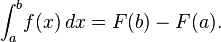
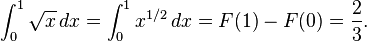
Approximations to integral of √
x from 0 to 1, with 5
■ (yellow) right endpoint partitions and 12
■ (green) left endpoint partitions
To start off, consider the curve y = f(x) between x = 0 and x = 1 with f(x) = √x. We ask:
-
What is the area under the function f, in the interval from 0 to 1?
and call this (yet unknown) area the integral of f. The notation for this integral will be
-

As a first approximation, look at the unit square given by the sides x = 0 to x = 1 and y = f(0) = 0 and y = f(1) = 1. Its area is exactly 1. As it is, the true value of the integral must be somewhat less. Decreasing the width of the approximation rectangles shall give a better result; so cross the interval in five steps, using the approximation points 0, 1/5, 2/5, and so on to 1. Fit a box for each step using the right end height of each curve piece, thus √(1⁄5), √(2⁄5), and so on to √1 = 1. Summing the areas of these rectangles, we get a better approximation for the sought integral, namely
-

We are taking a sum of finitely many function values of f, multiplied with the differences of two subsequent approximation points. We can easily see that the approximation is still too large. Using more steps produces a closer approximation, but will never be exact: replacing the 5 subintervals by twelve in the same way, but with the left end height of each piece, we will get an approximate value for the area of 0.6203, which is too small. The key idea is the transition from adding finitely many differences of approximation points multiplied by their respective function values to using infinitely many fine, or infinitesimal steps.
As for the actual calculation of integrals, the fundamental theorem of calculus, due to Newton and Leibniz, is the fundamental link between the operations of differentiating and integrating. Applied to the square root curve, f(x) = x1/2, it says to look at the antiderivative F(x) = (2/3)x3/2, and simply take F(1) − F(0), where 0 and 1 are the boundaries of the interval [0,1]. So the exact value of the area under the curve is computed formally as
-
(This is a case of a general rule, that for f(x) = xq, with q ≠ −1, the related function, the so-called antiderivative is F(x) = xq + 1/(q + 1).)
The notation
-

conceives the integral as a weighted sum, denoted by the elongated s, of function values, f(x), multiplied by infinitesimal step widths, the so-called differentials, denoted by dx. The multiplication sign is usually omitted.
Historically, after the failure of early efforts to rigorously interpret infinitesimals, Riemann formally defined integrals as a limit of weighted sums, so that the dx suggested the limit of a difference (namely, the interval width). Shortcomings of Riemann's dependence on intervals and continuity motivated newer definitions, especially the Lebesgue integral, which is founded on an ability to extend the idea of "measure" in much more flexible ways. Thus the notation
-

refers to a weighted sum in which the function values are partitioned, with μ measuring the weight to be assigned to each value. Here A denotes the region of integration.
Differential geometry, with its "calculus on manifolds", gives the familiar notation yet another interpretation. Now f(x) and dx become a differential form, ω = f(x) dx, a new differential operator d, known as the exterior derivative is introduced, and the fundamental theorem becomes the more general Stokes' theorem,
-
from which Green's theorem, the divergence theorem, and the fundamental theorem of calculus follow.
More recently, infinitesimals have reappeared with rigor, through modern innovations such as non-standard analysis. Not only do these methods vindicate the intuitions of the pioneers; they also lead to new mathematics.
Although there are differences between these conceptions of integral, there is considerable overlap. Thus, the area of the surface of the oval swimming pool can be handled as a geometric ellipse, a sum of infinitesimals, a Riemann integral, a Lebesgue integral, or as a manifold with a differential form. The calculated result will be the same for all.
Darboux upper sums of the function y = x2
Darboux lower sums of the function y = x2
Formal definitions
Integral example with irregular partitions (largest marked in red)
There are many ways of formally defining an integral, not all of which are equivalent. The differences exist mostly to deal with differing special cases which may not be integrable under other definitions, but also occasionally for pedagogical reasons. The most commonly used definitions of integral are Riemann integrals and Lebesgue integrals.
Riemann integral
The Riemann integral is defined in terms of Riemann sums of functions with respect to tagged partitions of an interval. Let [a,b] be a closed interval of the real line; then a tagged partition of [a,b] is a finite sequence
-

This partitions the interval [a,b] into n sub-intervals [xi−1, xi] indexed by i, each of which is "tagged" with a distinguished point ti ∈ [xi−1, xi]. A Riemann sum of a function f with respect to such a tagged partition is defined as
-

thus each term of the sum is the area of a rectangle with height equal to the function value at the distinguished point of the given sub-interval, and width the same as the sub-interval width. Let Δi = xi−xi−1 be the width of sub-interval i; then the mesh of such a tagged partition is the width of the largest sub-interval formed by the partition, maxi=1…n Δi. The Riemann integral of a function f over the interval [a,b] is equal to S if:
-
For all ε > 0 there exists δ > 0 such that, for any tagged partition [a,b] with mesh less than δ, we have
-

When the chosen tags give the maximum (respectively, minimum) value of each interval, the Riemann sum becomes an upper (respectively, lower) Darboux sum, suggesting the close connection between the Riemann integral and the Darboux integral.
Lebesgue integral
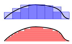
Riemann–Darboux's integration (top) and Lebesgue integration (bottom)
It is often of interest, both in theory and applications, to be able to pass to the limit under the integral. For instance, a sequence of functions can frequently be constructed that approximate, in a suitable sense, the solution to a problem. Then the integral of the solution function should be the limit of the integrals of the approximations. However, many functions that can be obtained as limits are not Riemann integrable, and so such limit theorems do not hold with the Riemann integral. Therefore it is of great importance to have a definition of the integral that allows a wider class of functions to be integrated (Rudin 1987).
Such an integral is the Lebesgue integral, that exploits the following fact to enlarge the class of integrable functions: if the values of a function are rearranged over the domain, the integral of a function should remain the same. Thus Henri Lebesgue introduced the integral bearing his name, explaining this integral thus in a letter to Paul Montel:
I have to pay a certain sum, which I have collected in my pocket. I take the bills and coins out of my pocket and give them to the creditor in the order I find them until I have reached the total sum. This is the Riemann integral. But I can proceed differently. After I have taken all the money out of my pocket I order the bills and coins according to identical values and then I pay the several heaps one after the other to the creditor. This is my integral.
-
Source: (Siegmund-Schultze 2008)
As Folland (1984, p. 56) puts it, "To compute the Riemann integral of f, one partitions the domain [a,b] into subintervals", while in the Lebesgue integral, "one is in effect partitioning the range of f". The definition of the Lebesgue integral thus begins with a measure, μ. In the simplest case, the Lebesgue measure μ(A) of an interval A = [a,b] is its width, b − a, so that the Lebesgue integral agrees with the (proper) Riemann integral when both exist. In more complicated cases, the sets being measured can be highly fragmented, with no continuity and no resemblance to intervals.
Using the "partitioning the range of f" philosophy, the integral of a non-negative function f : R → R should be the sum over t of the areas between a thin horizontal strip between y = t and y = t + dt. This area is just μ{ x : f(x) > t} dt. Let f∗(t) = μ{ x : f(x) > t}. The Lebesgue integral of f is then defined by (Lieb & Loss 2001)
-

where the integral on the right is an ordinary improper Riemann integral (f∗ is a strictly decreasing positive function, and therefore has a well-defined improper Riemann integral). For a suitable class of functions (the measurable functions) this defines the Lebesgue integral.
A general measurable function f is Lebesgue integrable if the area between the graph of f and the x-axis is finite:
-
In that case, the integral is, as in the Riemannian case, the difference between the area above the x-axis and the area below the x-axis:
-
where
-

Other integrals
Although the Riemann and Lebesgue integrals are the most widely used definitions of the integral, a number of others exist, including:
- The Darboux integral which is equivalent to a Riemann integral, meaning that a function is Darboux-integrable if and only if it is Riemann-integrable, and the values of the two integrals, if they exist, are equal. Darboux integrals have the advantage of being simpler to define than Riemann integrals.
- The Riemann–Stieltjes integral, an extension of the Riemann integral.
- The Lebesgue–Stieltjes integral, further developed by Johann Radon, which generalizes the Riemann–Stieltjes and Lebesgue integrals.
- The Daniell integral, which subsumes the Lebesgue integral and Lebesgue–Stieltjes integral without the dependence on measures.
- The Haar integral, used for integration on locally compact topological groups, introduced by Alfréd Haar in 1933.
- The Henstock–Kurzweil integral, variously defined by Arnaud Denjoy, Oskar Perron, and (most elegantly, as the gauge integral) Jaroslav Kurzweil, and developed by Ralph Henstock.
- The Itō integral and Stratonovich integral, which define integration with respect to semimartingales such as Brownian motion.
- The Young integral, which is a kind of Riemann–Stieltjes integral with respect to certain functions of unbounded variation.
- The rough path integral defined for functions equipped with some additional "rough path" structure, generalizing stochastic integration against both semimartingales and processes such as the fractional Brownian motion.
Properties
Linearity
- The collection of Riemann integrable functions on a closed interval [a, b] forms a vector space under the operations of pointwise addition and multiplication by a scalar, and the operation of integration
-
-
-
is a linear functional on this vector space. Thus, firstly, the collection of integrable functions is closed under taking linear combinations; and, secondly, the integral of a linear combination is the linear combination of the integrals,
-
-

- Similarly, the set of real-valued Lebesgue integrable functions on a given measure space E with measure μ is closed under taking linear combinations and hence form a vector space, and the Lebesgue integral
-
-

-
is a linear functional on this vector space, so that
-
-

-
-
-
that is compatible with linear combinations. In this situation the linearity holds for the subspace of functions whose integral is an element of V (i.e. "finite"). The most important special cases arise when K is R, C, or a finite extension of the field Qp of p-adic numbers, and V is a finite-dimensional vector space over K, and when K=C and V is a complex Hilbert space.
Linearity, together with some natural continuity properties and normalisation for a certain class of "simple" functions, may be used to give an alternative definition of the integral. This is the approach of Daniell for the case of real-valued functions on a set X, generalized by Nicolas Bourbaki to functions with values in a locally compact topological vector space. See (Hildebrandt 1953) for an axiomatic characterisation of the integral.
Inequalities for integrals
A number of general inequalities hold for Riemann-integrable functions defined on a closed and bounded interval [a, b] and can be generalized to other notions of integral (Lebesgue and Daniell).
- Upper and lower bounds. An integrable function f on [a, b], is necessarily bounded on that interval. Thus there are real numbers m and M so that m ≤ f (x) ≤ M for all x in [a, b]. Since the lower and upper sums of f over [a, b] are therefore bounded by, respectively, m(b − a) and M(b − a), it follows that
-
-

- Inequalities between functions. If f(x) ≤ g(x) for each x in [a, b] then each of the upper and lower sums of f is bounded above by the upper and lower sums, respectively, of g. Thus
-
-
-
This is a generalization of the above inequalities, as M(b − a) is the integral of the constant function with value M over [a, b].
-
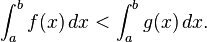
In addition, if the inequality between functions is strict, then the inequality between integrals is also strict. That is, if f(x) < g(x) for each x in [a, b], then
-
- Subintervals. If [c, d] is a subinterval of [a, b] and f(x) is non-negative for all x, then
-
-

-
-

-
If f is Riemann-integrable on [a, b] then the same is true for |f|, and
-

-
Moreover, if f and g are both Riemann-integrable then f 2, g 2, and fg are also Riemann-integrable, and
-

-
This inequality, known as the Cauchy–Schwarz inequality, plays a prominent role in Hilbert space theory, where the left hand side is interpreted as the inner product of two square-integrable functions f and g on the interval [a, b].
- Hölder's inequality. Suppose that p and q are two real numbers, 1 ≤ p, q ≤ ∞ with 1/p + 1/q = 1, and f and g are two Riemann-integrable functions. Then the functions |f|p and |g|q are also integrable and the following Hölder's inequality holds:
-
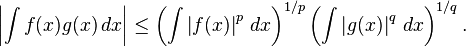
-
For p = q = 2, Hölder's inequality becomes the Cauchy–Schwarz inequality.
- Minkowski inequality. Suppose that p ≥ 1 is a real number and f and g are Riemann-integrable functions. Then |f|p, |g|p and |f + g|p are also Riemann integrable and the following Minkowski inequality holds:
-

-
An analogue of this inequality for Lebesgue integral is used in construction of Lp spaces.
Conventions
In this section f is a real-valued Riemann-integrable function. The integral
-

over an interval [a, b] is defined if a < b. This means that the upper and lower sums of the function f are evaluated on a partition a = x0 ≤ x1 ≤ . . . ≤ xn = b whose values xi are increasing. Geometrically, this signifies that integration takes place "left to right", evaluating f within intervals [x i , x i +1] where an interval with a higher index lies to the right of one with a lower index. The values a and b, the end-points of the interval, are called the limits of integration of f. Integrals can also be defined if a > b:
- Reversing limits of integration. If a > b then define
-
-
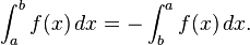
This, with a = b, implies:
- Integrals over intervals of length zero. If a is a real number then
-
-
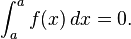
The first convention is necessary in consideration of taking integrals over subintervals of [a, b]; the second says that an integral taken over a degenerate interval, or a point, should be zero. One reason for the first convention is that the integrability of f on an interval [a, b] implies that f is integrable on any subinterval [c, d], but in particular integrals have the property that:
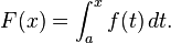
- Additivity of integration on intervals. If c is any element of [a, b], then
-
-

With the first convention the resulting relation
-
is then well-defined for any cyclic permutation of a, b, and c.
Instead of viewing the above as conventions, one can also adopt the point of view that integration is performed of differential forms on oriented manifolds only. If M is such an oriented m-dimensional manifold, and M' is the same manifold with opposed orientation and ω is an m-form, then one has:
-

These conventions correspond to interpreting the integrand as a differential form, integrated over a chain. In measure theory, by contrast, one interprets the integrand as a function f with respect to a measure  and integrates over a subset A, without any notion of orientation; one writes
 ![\textstyle{\int_A f\,d\mu = \int_{[a,b]} f\,d\mu}](https://upload.wikimedia.org/math/3/f/3/3f35814e537d2abecd5eada51fdc7bb7.png) to indicate integration over a subset A. This is a minor distinction in one dimension, but becomes subtler on higher dimensional manifolds; see Differential form: Relation with measures for details.
to indicate integration over a subset A. This is a minor distinction in one dimension, but becomes subtler on higher dimensional manifolds; see Differential form: Relation with measures for details.
Fundamental theorem of calculus
The fundamental theorem of calculus is the statement that differentiation and integration are inverse operations: if a continuous function is first integrated and then differentiated, the original function is retrieved. An important consequence, sometimes called the second fundamental theorem of calculus, allows one to compute integrals by using an antiderivative of the function to be integrated.
Statements of theorems
Fundamental theorem of calculus
Let f be a continuous real-valued function defined on a closed interval [a, b]. Let F be the function defined, for all x in [a, b], by
-
Then, F is continuous on [a, b], differentiable on the open interval (a, b), and
-
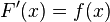
for all x in (a, b).
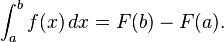
Second fundamental theorem of calculus
Let f be a real-valued function defined on a closed interval [a, b] that admits an antiderivative F on [a, b]. That is, f and F are functions such that for all x in [a, b],
-

If f is integrable on [a, b] then
-
Extensions
Improper integrals
A "proper" Riemann integral assumes the integrand is defined and finite on a closed and bounded interval, bracketed by the limits of integration. An improper integral occurs when one or more of these conditions is not satisfied. In some cases such integrals may be defined by considering the limit of a sequence of proper Riemann integrals on progressively larger intervals.
If the interval is unbounded, for instance at its upper end, then the improper integral is the limit as that endpoint goes to infinity.
-
If the integrand is only defined or finite on a half-open interval, for instance (a, b], then again a limit may provide a finite result.
-
That is, the improper integral is the limit of proper integrals as one endpoint of the interval of integration approaches either a specified real number, or ∞, or −∞. In more complicated cases, limits are required at both endpoints, or at interior points.
Consider, for example, the function  integrated from 0 to ∞ (shown right). At the lower bound, as x goes to 0 the function goes to ∞, and the upper bound is itself ∞, though the function goes to 0. Thus this is a doubly improper integral. Integrated, say, from 1 to 3, an ordinary Riemann sum suffices to produce a result of π/6. To integrate from 1 to ∞, a Riemann sum is not possible. However, any finite upper bound, say t (with t > 1), gives a well-defined result,
  . This has a finite limit as t goes to infinity, namely π/2. Similarly, the integral from 1/3 to 1 allows a Riemann sum as well, coincidentally again producing π/6. Replacing 1/3 by an arbitrary positive value s (with s < 1) is equally safe, giving
  . This, too, has a finite limit as s goes to zero, namely π/2. Combining the limits of the two fragments, the result of this improper integral is
-

This process does not guarantee success; a limit might fail to exist, or might be unbounded. For example, over the bounded interval from 0 to 1 the integral of 1/x does not converge; and over the unbounded interval from 1 to ∞ the integral of  does not converge.
It might also happen that an integrand is unbounded at an interior point, in which case the integral must be split at that point. For the integral as a whole to converge, the limit integrals on both sides must exist and must be bounded. For example:
-
![\begin{align}
\int_{-1}^{1} \frac{dx}{\sqrt[3]{x^2}} &{} = \lim_{s \to 0} \int_{-1}^{-s} \frac{dx}{\sqrt[3]{x^2}}
+ \lim_{t \to 0} \int_{t}^{1} \frac{dx}{\sqrt[3]{x^2}} \\
&{} = \lim_{s \to 0} 3(1-\sqrt[3]{s}) + \lim_{t \to 0} 3(1-\sqrt[3]{t}) \\
&{} = 3 + 3 \\
&{} = 6.
\end{align}](https://upload.wikimedia.org/math/c/a/0/ca0a80817e0cb2c5bdbd93559e4383f5.png)
But the similar integral
-

cannot be assigned a value in this way, as the integrals above and below zero do not independently converge. (However, see Cauchy principal value.)
Multiple integration

Double integral as volume under a surface.
Integrals can be taken over regions other than intervals. In general, an integral over a set E of a function f is written:
-

Here x need not be a real number, but can be another suitable quantity, for instance, a vector in R3. Fubini's theorem shows that such integrals can be rewritten as an iterated integral. In other words, the integral can be calculated by integrating one coordinate at a time.
Just as the definite integral of a positive function of one variable represents the area of the region between the graph of the function and the x-axis, the double integral of a positive function of two variables represents the volume of the region between the surface defined by the function and the plane which contains its domain. (The same volume can be obtained via the triple integral — the integral of a function in three variables — of the constant function f(x, y, z) = 1 over the above mentioned region between the surface and the plane.) If the number of variables is higher, then the integral represents a hypervolume, a volume of a solid of more than three dimensions that cannot be graphed.
For example, the volume of the cuboid of sides 4 × 6 × 5 may be obtained in two ways:
-
-
-
of the function f(x, y) = 5 calculated in the region D in the xy-plane which is the base of the cuboid. For example, if a rectangular base of such a cuboid is given via the xy inequalities 3 ≤ x ≤ 7, 4 ≤ y ≤ 10, our above double integral now reads
-
-
![\int_4^{10}\left[ \int_3^7 \ 5 \ dx\right] dy.](https://upload.wikimedia.org/math/e/d/3/ed391d60d495500c364c5d696423d9f0.png)
-
From here, integration is conducted with respect to either x or y first; in this example, integration is first done with respect to x as the interval corresponding to x is the inner integral. Once the first integration is completed via the
 method or otherwise, the result is again integrated with respect to the other variable. The result will equate to the volume under the surface.
-
-

-
of the constant function 1 calculated on the cuboid itself.
Line integrals
Main article:
Line integral
A line integral sums together elements along a curve.
The concept of an integral can be extended to more general domains of integration, such as curved lines and surfaces. Such integrals are known as line integrals and surface integrals respectively. These have important applications in physics, as when dealing with vector fields.
A line integral (sometimes called a path integral) is an integral where the function to be integrated is evaluated along a curve. Various different line integrals are in use. In the case of a closed curve it is also called a contour integral.
The function to be integrated may be a scalar field or a vector field. The value of the line integral is the sum of values of the field at all points on the curve, weighted by some scalar function on the curve (commonly arc length or, for a vector field, the scalar product of the vector field with a differential vector in the curve). This weighting distinguishes the line integral from simpler integrals defined on intervals. Many simple formulas in physics have natural continuous analogs in terms of line integrals; for example, the fact that work is equal to force, F, multiplied by displacement, s, may be expressed (in terms of vector quantities) as:
-

For an object moving along a path C in a vector field F such as an electric field or gravitational field, the total work done by the field on the object is obtained by summing up the differential work done in moving from s to s + ds. This gives the line integral
-
Surface integrals

The definition of surface integral relies on splitting the surface into small surface elements.
A surface integral is a definite integral taken over a surface (which may be a curved set in space); it can be thought of as the double integral analog of the line integral. The function to be integrated may be a scalar field or a vector field. The value of the surface integral is the sum of the field at all points on the surface. This can be achieved by splitting the surface into surface elements, which provide the partitioning for Riemann sums.
For an example of applications of surface integrals, consider a vector field v on a surface S; that is, for each point x in S, v(x) is a vector. Imagine that we have a fluid flowing through S, such that v(x) determines the velocity of the fluid at x. The flux is defined as the quantity of fluid flowing through S in unit amount of time. To find the flux, we need to take the dot product of v with the unit surface normal to S at each point, which will give us a scalar field, which we integrate over the surface:
-

The fluid flux in this example may be from a physical fluid such as water or air, or from electrical or magnetic flux. Thus surface integrals have applications in physics, particularly with the classical theory of electromagnetism.
Integrals of differential forms
A differential form is a mathematical concept in the fields of multivariable calculus, differential topology and tensors. The modern notation for the differential form, as well as the idea of the differential forms as being the wedge products of exterior derivatives forming an exterior algebra, was introduced by Élie Cartan.
We initially work in an open set in Rn. A 0-form is defined to be a smooth function f. When we integrate a function f over an m-dimensional subspace S of Rn, we write it as
-
(The superscripts are indices, not exponents.) We can consider dx1 through dxn to be formal objects themselves, rather than tags appended to make integrals look like Riemann sums. Alternatively, we can view them as covectors, and thus a measure of "density" (hence integrable in a general sense). We call the dx1, …, dxn basic 1-forms.
We define the wedge product, "∧", a bilinear "multiplication" operator on these elements, with the alternating property that
-

for all indices a. Alternation along with linearity and associativity implies dxb∧dxa = −dxa∧dxb. This also ensures that the result of the wedge product has an orientation.
We define the set of all these products to be basic 2-forms, and similarly we define the set of products of the form dxa∧dxb∧dxc to be basic 3-forms. A general k-form is then a weighted sum of basic k-forms, where the weights are the smooth functions f. Together these form a vector space with basic k-forms as the basis vectors, and 0-forms (smooth functions) as the field of scalars. The wedge product then extends to k-forms in the natural way. Over Rn at most n covectors can be linearly independent, thus a k-form with k > n will always be zero, by the alternating property.
In addition to the wedge product, there is also the exterior derivative operator d. This operator maps k-forms to (k+1)-forms. For a k-form ω = f dxa over Rn, we define the action of d by:
-

with extension to general k-forms occurring linearly.
This more general approach allows for a more natural coordinate-free approach to integration on manifolds. It also allows for a natural generalisation of the fundamental theorem of calculus, called Stokes' theorem, which we may state as
-

where ω is a general k-form, and ∂Ω denotes the boundary of the region Ω. Thus, in the case that ω is a 0-form and Ω is a closed interval of the real line, this reduces to the fundamental theorem of calculus. In the case that ω is a 1-form and Ω is a two-dimensional region in the plane, the theorem reduces to Green's theorem. Similarly, using 2-forms, and 3-forms and Hodge duality, we can arrive at Stokes' theorem and the divergence theorem. In this way we can see that differential forms provide a powerful unifying view of integration.
Summations
The discrete equivalent of integration is summation. Summations and integrals can be put on the same foundations using the theory of Lebesgue integrals or time scale calculus.
Methods for computing integrals
Analytical
The most basic technique for computing definite integrals of one real variable is based on the fundamental theorem of calculus. Let f(x) be the function of x to be integrated over a given interval [a, b]. Then, find an antiderivative of f; that is, a function F such that F' = f on the interval. Provided the integrand and integral have no singularities on the path of integration, by the fundamental theorem of calculus,
-
The integral is not actually the antiderivative, but the fundamental theorem provides a way to use antiderivatives to evaluate definite integrals.
The most difficult step is usually to find the antiderivative of f. It is rarely possible to glance at a function and write down its antiderivative. More often, it is necessary to use one of the many techniques that have been developed to evaluate integrals. Most of these techniques rewrite one integral as a different one which is hopefully more tractable. Techniques include:
Alternate methods exist to compute more complex integrals. Many nonelementary integrals can be expanded in a Taylor series and integrated term by term. Occasionally, the resulting infinite series can be summed analytically. The method of convolution using Meijer G-functions can also be used, assuming that the integrand can be written as a product of Meijer G-functions. There are also many less common ways of calculating definite integrals; for instance, Parseval's identity can be used to transform an integral over a rectangular region into an infinite sum. Occasionally, an integral can be evaluated by a trick; for an example of this, see Gaussian integral.
Computations of volumes of solids of revolution can usually be done with disk integration or shell integration.
Specific results which have been worked out by various techniques are collected in the list of integrals.
Symbolic
Many problems in mathematics, physics, and engineering involve integration where an explicit formula for the integral is desired. Extensive tables of integrals have been compiled and published over the years for this purpose. With the spread of computers, many professionals, educators, and students have turned to computer algebra systems that are specifically designed to perform difficult or tedious tasks, including integration. Symbolic integration has been one of the motivations for the development of the first such systems, like Macsyma.
A major mathematical difficulty in symbolic integration is that in many cases, a closed formula for the antiderivative of a rather simple-looking function does not exist. For instance, it is known that the antiderivatives of the functions exp(x2), xx and (sin x)/x cannot be expressed in the closed form involving only rational and exponential functions, logarithm, trigonometric and inverse trigonometric functions, and the operations of multiplication and composition; in other words, none of the three given functions is integrable in elementary functions, which are the functions which may be built from rational functions, roots of a polynomial, logarithm, and exponential functions. The Risch algorithm provides a general criterion to determine whether the antiderivative of an elementary function is elementary, and, if it is, to compute it. Unfortunately, it turns out that functions with closed expressions of antiderivatives are the exception rather than the rule. Consequently, computerized algebra systems have no hope of being able to find an antiderivative for a randomly constructed elementary function. On the positive side, if the 'building blocks' for antiderivatives are fixed in advance, it may be still be possible to decide whether the antiderivative of a given function can be expressed using these blocks and operations of multiplication and composition, and to find the symbolic answer whenever it exists. The Risch algorithm, implemented in Mathematica and other computer algebra systems, does just that for functions and antiderivatives built from rational functions, radicals, logarithm, and exponential functions.
Some special integrands occur often enough to warrant special study. In particular, it may be useful to have, in the set of antiderivatives, the special functions of physics (like the Legendre functions, the hypergeometric function, the Gamma function, the Incomplete Gamma function and so on — see Symbolic integration for more details). Extending the Risch's algorithm to include such functions is possible but challenging and has been an active research subject.
More recently a new approach has emerged, using D-finite function, which are the solutions of linear differential equations with polynomial coefficients. Most of the elementary and special functions are D-finite and the integral of a D-finite function is also a D-finite function. This provide an algorithm to express the antiderivative of a D-finite function as the solution of a differential equation.
This theory allows also to compute a definite integrals of a D-function as the sum of a series given by the first coefficients and an algorithm to compute any coefficient.[1]
Numerical
The integrals encountered in a basic calculus course are deliberately chosen for simplicity; those found in real applications are not always so accommodating. Some integrals cannot be found exactly, some require special functions which themselves are a challenge to compute, and others are so complex that finding the exact answer is too slow. This motivates the study and application of numerical methods for approximating integrals, which today use floating-point arithmetic on digital electronic computers. Many of the ideas arose much earlier, for hand calculations; but the speed of general-purpose computers like the ENIAC created a need for improvements.
The goals of numerical integration are accuracy, reliability, efficiency, and generality. Sophisticated methods can vastly outperform a naive method by all four measures (Dahlquist & Björck 2008; Kahaner, Moler & Nash 1989; Stoer & Bulirsch 2002). Consider, for example, the integral
-

which has the exact answer 94/25 = 3.76. (In ordinary practice the answer is not known in advance, so an important task — not explored here — is to decide when an approximation is good enough.) A “calculus book” approach divides the integration range into, say, 16 equal pieces, and computes function values.
-
Spaced function values
| x |
−2.00 |
−1.50 |
−1.00 |
−0.50 |
0.00 |
0.50 |
1.00 |
1.50 |
2.00 |
| f(x) |
2.22800 |
2.45663 |
2.67200 |
2.32475 |
0.64400 |
−0.92575 |
−0.94000 |
−0.16963 |
0.83600 |
| x |
|
−1.75 |
−1.25 |
−0.75 |
−0.25 |
0.25 |
0.75 |
1.25 |
1.75 |
|
| f(x) |
|
2.33041 |
2.58562 |
2.62934 |
1.64019 |
−0.32444 |
−1.09159 |
−0.60387 |
0.31734 |
|
| |
|
|
|
|
|
|
|
|
|
|
|
|
|
|
|
|
|
|

Numerical quadrature methods:
■ Rectangle,
■ Trapezoid,
■ Romberg,
■ Gauss
Using the left end of each piece, the rectangle method sums 16 function values and multiplies by the step width, h, here 0.25, to get an approximate value of 3.94325 for the integral. The accuracy is not impressive, but calculus formally uses pieces of infinitesimal width, so initially this may seem little cause for concern. Indeed, repeatedly doubling the number of steps eventually produces an approximation of 3.76001. However, 218 pieces are required, a great computational expense for such little accuracy; and a reach for greater accuracy can force steps so small that arithmetic precision becomes an obstacle.
A better approach replaces the horizontal tops of the rectangles with slanted tops touching the function at the ends of each piece. This trapezium rule is almost as easy to calculate; it sums all 17 function values, but weights the first and last by one half, and again multiplies by the step width. This immediately improves the approximation to 3.76925, which is noticeably more accurate. Furthermore, only 210 pieces are needed to achieve 3.76000, substantially less computation than the rectangle method for comparable accuracy.
Romberg's method builds on the trapezoid method to great effect. First, the step lengths are halved incrementally, giving trapezoid approximations denoted by T(h0), T(h1), and so on, where hk+1 is half of hk. For each new step size, only half the new function values need to be computed; the others carry over from the previous size (as shown in the table above). But the really powerful idea is to interpolate a polynomial through the approximations, and extrapolate to T(0). With this method a numerically exact answer here requires only four pieces (five function values)! The Lagrange polynomial interpolating {hk,T(hk)}k = 0…2 = {(4.00,6.128), (2.00,4.352), (1.00,3.908)} is 3.76 + 0.148h2, producing the extrapolated value 3.76 at h = 0.
Gaussian quadrature often requires noticeably less work for superior accuracy. In this example, it can compute the function values at just two x positions, ±2⁄√3, then double each value and sum to get the numerically exact answer. The explanation for this dramatic success lies in error analysis, and a little luck. An n-point Gaussian method is exact for polynomials of degree up to 2n−1. The function in this example is a degree 3 polynomial, plus a term that cancels because the chosen endpoints are symmetric around zero. (Cancellation also benefits the Romberg method.)
Shifting the range left a little, so the integral is from −2.25 to 1.75, removes the symmetry. Nevertheless, the trapezoid method is rather slow, the polynomial interpolation method of Romberg is acceptable, and the Gaussian method requires the least work — if the number of points is known in advance. As well, rational interpolation can use the same trapezoid evaluations as the Romberg method to greater effect.
-
Quadrature method cost comparison
| Method |
Trapezoid |
Romberg |
Rational |
Gauss |
| Points |
1048577 |
257 |
129 |
36 |
| Rel. Err. |
−5.3×10⁻¹³ |
−6.3×10⁻¹⁵ |
8.8×10⁻¹⁵ |
3.1×10⁻¹⁵ |
| Value |
 |
In practice, each method must use extra evaluations to ensure an error bound on an unknown function; this tends to offset some of the advantage of the pure Gaussian method, and motivates the popular Gauss–Kronrod quadrature formulae. Symmetry can still be exploited by splitting this integral into two ranges, from −2.25 to −1.75 (no symmetry), and from −1.75 to 1.75 (symmetry). More broadly, adaptive quadrature partitions a range into pieces based on function properties, so that data points are concentrated where they are needed most.
Simpson's rule, named for Thomas Simpson (1710–1761), uses a parabolic curve to approximate integrals. In many cases, it is more accurate than the trapezoidal rule and others. The rule states that
-
![\int_a^b f(x) \, dx \approx \frac{b-a}{6}\left[f(a) + 4f\left(\frac{a+b}{2}\right)+f(b)\right],](https://upload.wikimedia.org/math/c/0/5/c05540185f59fddd30daa081d2bd9b27.png)
with an error of
-
The computation of higher-dimensional integrals (for example, volume calculations) makes important use of such alternatives as Monte Carlo integration.
A calculus text is no substitute for numerical analysis, but the reverse is also true. Even the best adaptive numerical code sometimes requires a user to help with the more demanding integrals. For example, improper integrals may require a change of variable or methods that can avoid infinite function values, and known properties like symmetry and periodicity may provide critical leverage.
Mechanical
The area of an arbitrary two-dimensional shape can be determined using a measuring instrument called planimeter. The volume of irregular objects can be measured with precision by the fluid displaced as the object is submerged; see Archimedes's Eureka.
Geometrical
Area can be found via geometrical compass-and-straightedge constructions of an equivalent square, e.g., squaring the circle.
Some important definite integrals
Mathematicians have used definite integrals as a tool to define identities. Among these identities is the definition of the Euler–Mascheroni constant:
-

the Gamma function:
-

the Fourier transform which is widely used in physics:
-
Laplace transform which is widely used in engineering:
-
and the Gaussian Integral fundamental to the Normal Distribution used in probability and statistics:


 ,
,  atau kadang-kadang, jika asas
  .
. (ditulis
  sama dengan 2, kerana
  . Logaritma asli bagi
  ) ialah 1 kerana
  , manakala logaritma asli bagi 1 (
 ) ialah 0, kerana

 dari 1 ke
  dari 1 ke
  , iaitu kamiran,

 seperti berikut:
 .
. . Oleh kerana julat fungsi eksponen bagi argumen-argumen nyata ialah semua nombor nyata positif, dan fungsi eksponen meningkat secara khusus, yang demikian adalah tertakrif rapi bagi semua
 (lihat


 .
.
 ) jika


 R terdefinisi pada garis
  R maka kita menyebut limit f ketika x mendekati p adalah L, yang ditulis sebagai:


![\int_{-1}^{1} \frac{dx}{\sqrt[3]{x^2}} = 6](https://upload.wikimedia.org/math/c/4/2/c42bd4cc4fe5f36fe150f31308e79124.png)


